Profiling an MPI program with MAP
- Objectives
- MAP profiler
- Code example
- Using MAP to profile an executable
- Interpreting the profiling data
- Exercises
Objectives
You will:
- learn how to use MAP to profile a parallel MPI code
- learn how to interpret the profiling data
MAP profiler
On NeSI systems the Arm MAP profiler is provided as part of the forge module (along with the parallel debugger DDT).
MAP is a commercial product, which can profile parallel, multi-threaded and single-threaded C/C++, Fortran, as well as Python code. It can be used without code modification.
MAP can be used to identify hotspots and load balance problems in parallel codes. In contrast to the cProfiler described in here, MAP can be used to instrument Python, C, C++ and Fortran codes. In contrast to other profilers, there is no need to recompile the code and MAP supports OpenMP threads and/or MPI communication. It comes with a graphical user interface which makes it easy to drill down into particular code sections or focus on specific time intervals during the run.
For more details see the Arm MAP documentation.
Code example
We’ll use the scatter.py code in directory mpi of the solutions branch. Start by
git fetch --all
git checkout solutions
cd mpi
Using MAP to profile an executable
To use MAP we need to load the forge module in our batch script and add map --profile in front of the executable. See for example
ml forge
map --profile srun python scatter.py
in the Slurm script “scatter_map.sl”.
Upon execution, a file with subscript .map will be generated. The results can be viewed, for instance, with
map python3_scatter_py_4p_1n_1t_2019-05-22_00-58.map
(the .map file name will vary with each run.) See section MAP Profile for how to interpret the results.
Note: command map --profile must precede “srun” in the case of an MPI program. For serial or OpenMP programs we recommend “map” and its options to be after “srun”.
Interpreting the profiling data
Upon execution, a file with subscript .map will be generated. The results can be viewed with the command map, for instance
map python3_scatter_py_8p_1n_2019-01-14_00-31.map
(the .map file name will vary with each run.)
The profile window is divided into three main sections (click on picture to enlarge).
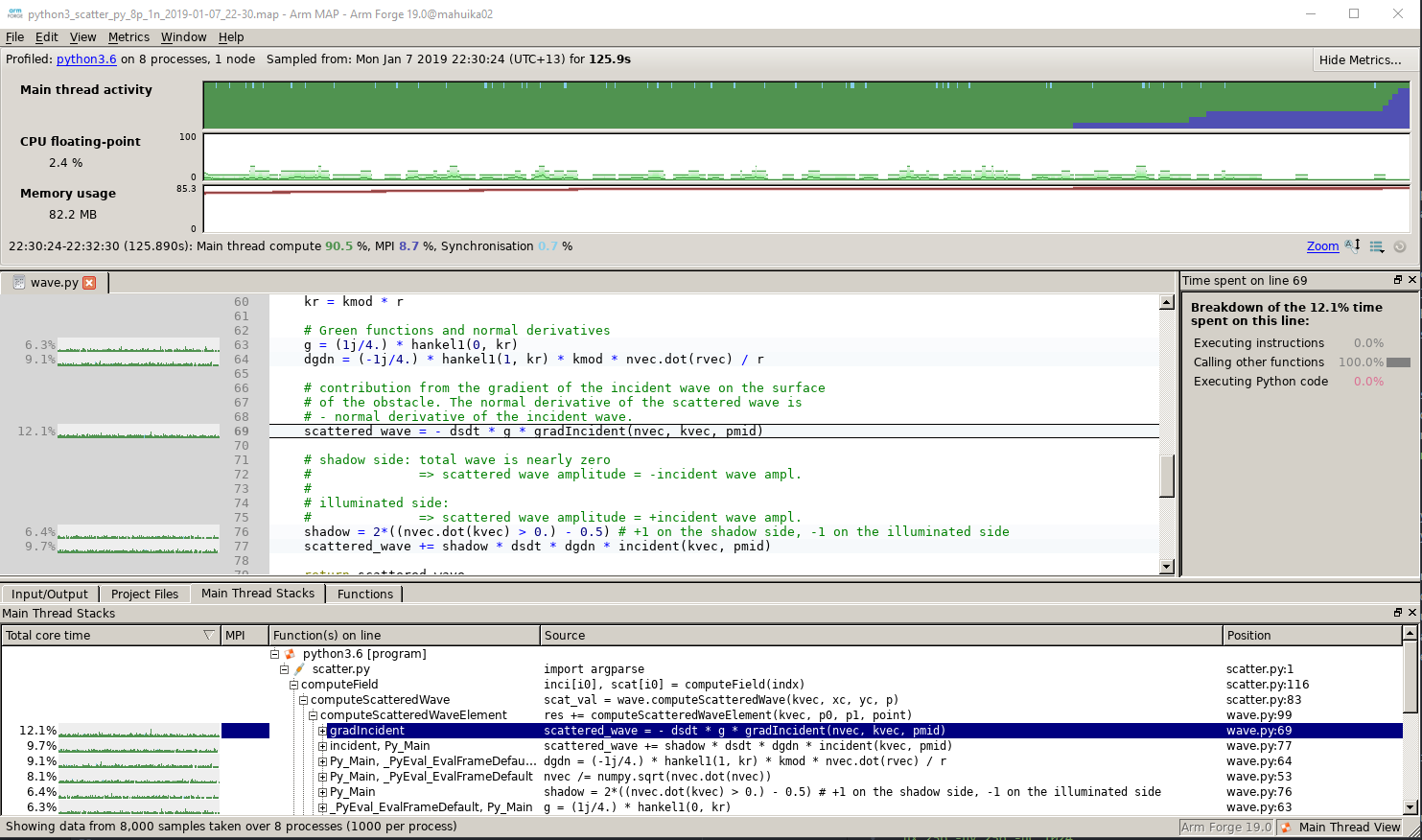
On top, various metrics can be selected in the “Metrics” menu. In the middle part, a source code navigator connects line by line with profiling data. Most interesting is the profiling table at the bottom, which sorts the most time consuming parts of the program, providing function names, source code and line numbers.
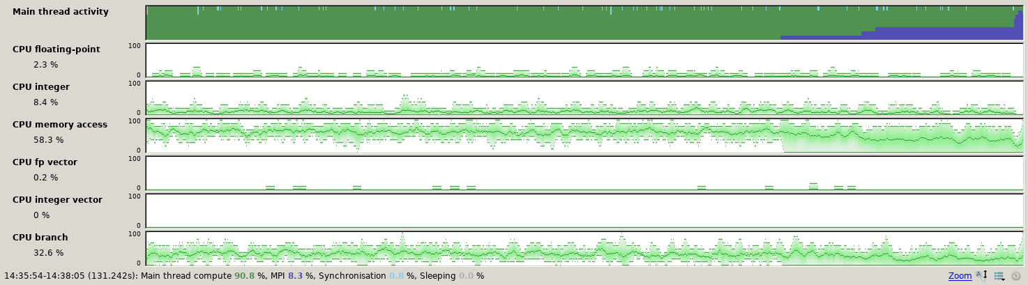
The Metrics part can be changed to:
- Activity timeline
- CPU instructions
- CPU Time
- IO
- Memory
- MPI
As an example, “CPU instructions” present the usage of different instruction sets during the program run time.
Exercises
- profile the scatter code under the mpi directory:
- use 16 MPI tasks
- increase the problem size to
-nx 256 -ny 256 -nc 256to make the test run longer- what is the amount of time spent in
computeScatteredWavefor the above test case?