Profiling with Python tools
- Objectives
- Profiling Python code with cProfile
- Profiling Python code with line_profiler
- Memory Profiler
- Exercises
Objectives
You will:
- learn how to gather profiling data using cProfile
- learn how to visualise profiling data
- learn how to interpret profiling data
Here we’ll profile the scatter code to identify the sections of the code where most the execution time is spent.
We’ll use the code in directory original. Start with the command
cd original
Profiling Python code with cProfile
The cProfile profiler is one implementation of the Python profiling interface. It measures the time spent within functions and the number of calls made to them.
Note: The timing information should not be taken as absolute values, since the profiling itself could possibly extend the run time in some cases.
Run the following command to profile the code:
Replace python scatter.py with
python -m cProfile -o output.pstats scatter.py
in your Slurm script or when running interactively. Additional arguments can be passed to the scatter.py at the end if needed.
Notice the two options in the above command.
- -m cProfile : the -m option specifies the python module to run as a script - this allows us to run cProfile from the command-line
- -o output.pstats : the -o option specifies that the profiling results be written to the named file
If you leave out these options the code will just run normally.
A nice way to visualise the output.pstats file is with gprof2dot.
Visualising the profiling output with gprof2dot
Note: You will need programs gprof2dot and dot, which are available on Mahuika and Maui. On other systems, use conda install gprof2dot to install gprof2dot and conda install graphviz to install Graphviz which provides the dot command.
Run gprof2dot to generate a PNG image file:
gprof2dot --colour-nodes-by-selftime -f pstats output.pstats | \
    dot -Tpng -o output.png
On Maui, generate an EPS image
gprof2dot --colour-nodes-by-selftime -f pstats output.pstats | \
    dot -Teps -o output.eps
as you would otherwise get message Format: "png" not recognized.
Now view output.png with the command display output.png on Mahuika (or display output.eps on Maui)
if you have enabled X11-forwarding in your
ssh command. Alternatively, you can copy the file your local machine and open it there.
The image should look something like this:
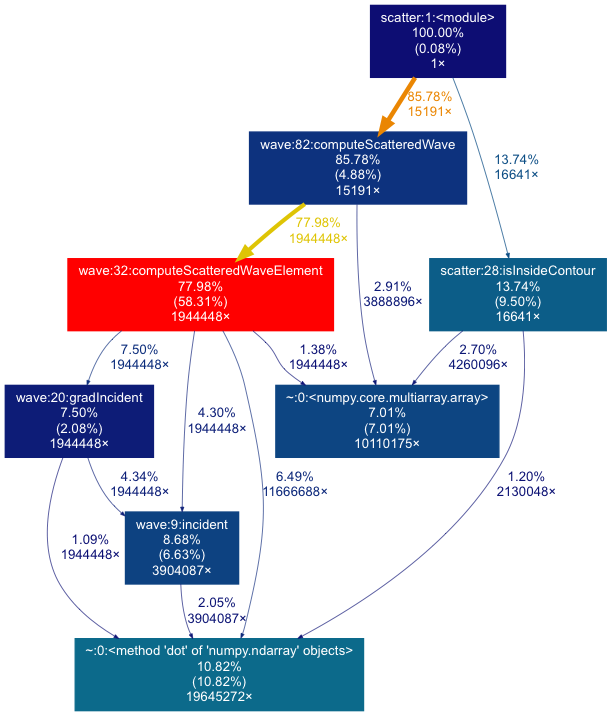
Interpreting the gprof2dot output
What the image shows:
- Each box represents a function from the input file, and contains information on:
- the percentage of total run time spent in this function, including time spent in other functions that are called by this function
- (in brackets) the percentage of total run time spent in this function only, i.e. excluding time spent in other functions that are called by this function. We call this self time
- the number of times this function was called
- Arrows indicate which functions are called by other functions
- information about the number of times called and percentage of total run time
- We used the option
--colour-nodes-by-selftime, so boxes are coloured by self time (the number in brackets)- red coloured boxes correspond to functions where the most time is spent
- blue boxes correspond to functions where the least time is spent
- Some functions that take a very low percentage of total run time may not show up
What to look for:
- Typically you would look for functions that have a lot of self time (the
number in brackets). We call these functions hotspots.
- 58.31% of total time is spent in
computeScatteredWaveElement(the red box), so this would be a good place to start when trying to optimise this code.
- 58.31% of total time is spent in
- Sometimes functions show up from libraries that you call (e.g. scipy or
numpy), for example the green box calling
dotthat takes 10.82% total time.- Usually you don’t want to change code from external libraries, but you can see which of your functions call an external library function by going back along the arrow from that function. You might be able to optimise the way your code calls the external function, use a more optimised library, or remove the call entirely.
Profiling Python code with line_profiler
The cProfile tool only times function calls. This is a good first step to find hotspots in your code (and often this is enough by itself). However, in some cases knowing that a particular function takes a lot of time is not particularly helpful. For example, it could be a very long function with multiple loops and computations.
line_profiler is a python profiler for doing line-by-line profiling. Typically, you would use line_profiler to gather more information about functions that cProfile has identified as hotspots. To use it, you modify the source code of your python file slightly to specify which functions are to be profiled. line_profiler will time the execution of individual lines within these designated functions.
Note: line_profiler is installed in the Python module we loaded earlier.
You can check that it is installed by running kernprof --help, which should print
help information for the kernprof (line_profiler) program that we are going
to use. (If not then pip install line_profiler.)
To demonstrate the use of line_profiler we will use it to profile the
isInsideContour function in the file scatter.py.
Note: we choose this function because it is short, which means we can include the output here and explain it.
- Edit the file scatter.py. Find the line that starts with:
def isInsideContour(p, xc, yc):On the previous line add
@profile, which is known as a decorator and tells line_profiler that we want to profile this function:@profile def isInsideContour(p, xc, yc): - Run line_profiler:
kernprof -l -v scatter.pyThe
-lflag tells line_profiler to do line-by-line profiling and-vtells it to print the profiling information out at the end of the run.
Detailed documentation about line_profiler can be found here.
Interpreting line_profiler output
You should see something like this after line_profiler has run:
Wrote profile results to scatter.py.lprof
Timer unit: 1e-06 s

Total time: 13.3867 s
File: scatter.py
Function: isInsideContour at line 28

Line #      Hits         Time  Per Hit   % Time  Line Contents
==============================================================
    28                                           @profile
    29                                           def isInsideContour(p, xc, yc):
    30                                               """
    31                                               Check if a point is inside closed contour
    32
    33                                               @param p point (2d array)
    34                                               @param xc array of x points, anticlockwise and must close
    35                                               @param yc array of y points, anticlockwise and must close
    36                                               @return True if p is inside, False otherwise
    37                                               """
    38     16641      12437.0      0.7      0.1      inside = True
    39   2146689     741826.0      0.3      5.5      for i0 in range(len(xc) - 1):
    40   2130048     766306.0      0.4      5.7          i1 = i0 + 1
    41   2130048    4790410.0      2.2     35.8          a = numpy.array([xc[i0], yc[i0]]) - p[:2]
    42   2130048    4702409.0      2.2     35.1          b = numpy.array([xc[i1], yc[i1]]) - p[:2]
    43                                                   # point is outside if any of the triangle extending from the point to the segment
    44                                                   # has negative area (cross product < 0)
    45                                                   # count a point on the contour as being outside (cross product == 0)
    46   2130048    2367141.0      1.1     17.7          inside &= (a[0]*b[1] - a[1]*b[0] > 1.e-10)
    47     16641       6180.0      0.4      0.0      return inside
- Line numbers and the contents of each line are shown
- The “% Time” column is useful; it shows the percentage of time in that function that was spent on that line. Here lines 41-42 dominate.
- “Hits” shows the number of times that line was run
- We can see that lines 41, 42 and 46 each take around 35%, 35% and 17% of the time spent in this function respectively.
Memory Profiler
There is another useful Python profiling tool called memory_profiler,
which can monitor memory consumption in a Python script on a line-by-line basis.
The memory profiler tool is used in a similar way to the line_profiler tool we
already covered, i.e. you have to use the @profile decorator to explicitly
tell memory_profiler which functions you wish to profile.
We will not cover memory profiler in detail here but more information can be found at the page linked above.
Exercises
- how much self time in percent is spent in
computeScatteredWave?- how much total time in percent is spent in
computeScatteredWave?- does it make sense to focus optimisation efforts on
computeScatteredWave?