MPI parallelism
- Objectives
- What is MPI
- An example of MPI work load distribution
- Running the scatter code using multiple MPI processes
- How to use MPI to accelerate scatter.py
- Exercises
Objectives
You will:
- learn what MPI is
- how to parallelise code, and in particular:
- learn how to disribute the work load among processes
- how to gather the results computed on separate processes
What is MPI
MPI is a standard application programming interface for creating and executing parallel programs. MPI was originally written for C, C++ and Fortran code but implementations have since become available for a variety of other languages, including Python.
MPI programs are started as a bunch of instances (often called “processes” or “tasks”) of an executable, which run concurrently.
As each process runs, the program may need to exchange data (“messages” - hence the name) with other processes. An example of data exchanges is point-to-point communication where one process sends data to another process. In other cases data may be “gathered” from multiple processes at once and sent to a root process. Inversely, data can be “scattered” from the root process to multiple other processes in one step.
Pros
- suitable for anything from laptops to supercomputers with hundreds of thousands of cores
- unlike shared memory approaches like OpenMP, MPI code can utilise resources beyond a single node
- can be used in combination with OpenMP and other parallelisation methods
Cons
- there are no serial sections in MPI code and hence MPI programs need to be written to run in parallel from the beginning to the end
- some algorithms are difficult to implement efficiently with MPI due its distributed memory approach and communication overhead
- it is easy to create “dead locks” where one or more processes get stuck waiting for a message
- the requested computing resources are occupied the whole run time, i.e. there is no dynamic allocation/deallocation of CPU cores
An example of MPI work load distribution
Let’s revisit our multiprocessing problem where we fill in an array by calling an expensive function
import time

def f(x):
	# expensive function
	time.sleep(10)
	return x

# call the function sequentially for input values 0, 1, 2, 3 and 4
input_values = [x for x in range(5)]
res = [f(x) for x in input_values]
Further let’s assume that we have 3 processes to compute the 5 elements of our problem. To distribute the work load, each process will compute a few elements of the array. Process 0 will compute the first two elements, process 1 the next two elements, etc. until the last process which will be computing the remaining element. Once the elements of the array are computed, a gather operation collects the results into a single array on the last process. This is shown below with process 0 in red, process 1 in blue and process 2 in yellow.
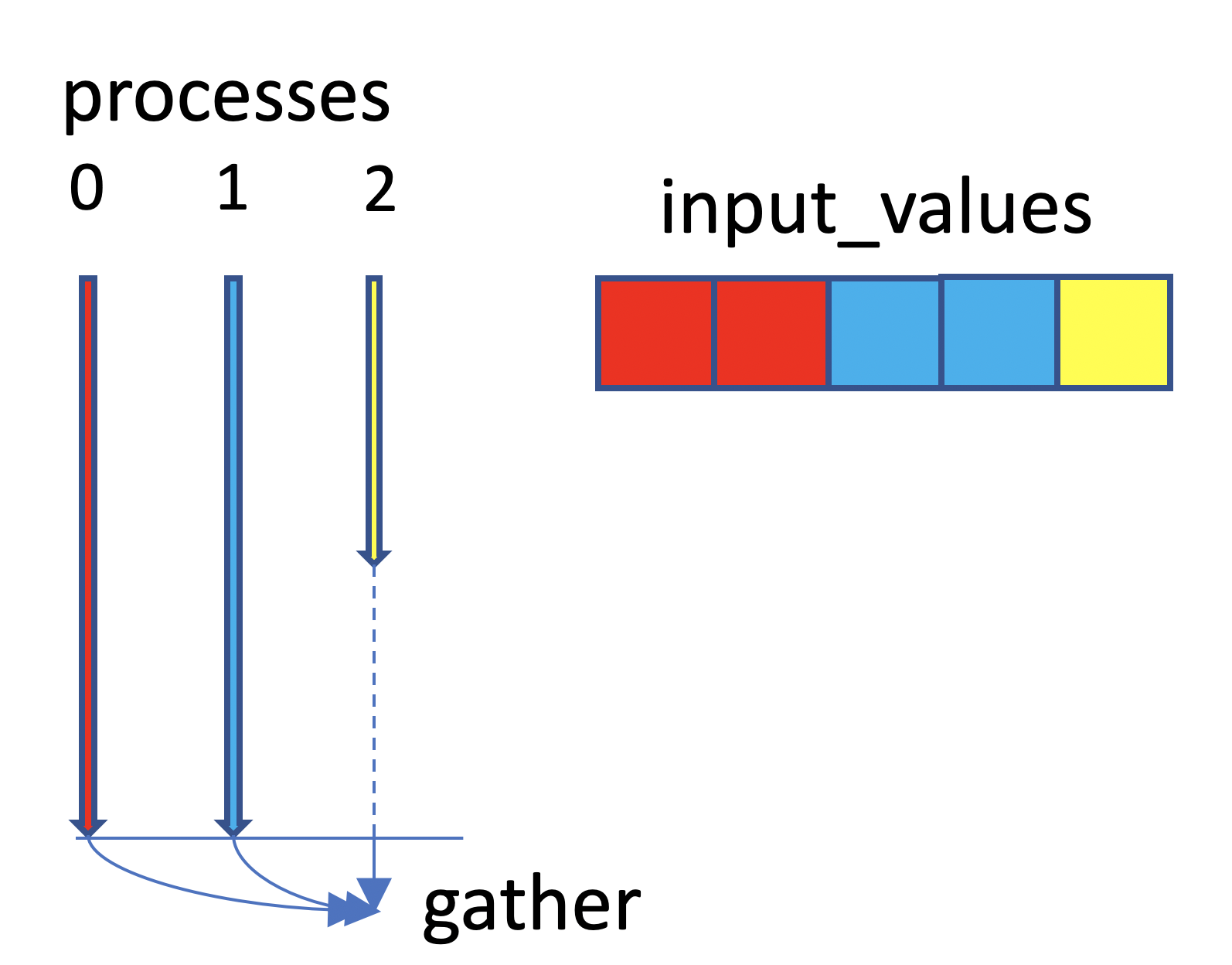
Neglecting the time it takes to gather the results, we can expect the execution time to be reduced from 5 time units (number of elements) to 2 time units (maximum number of elements handled by a process). Thus we get a speedup of 5/2 = 2.5x in this case. The ideal speedup is 3x but this cannot happen because process 2 has to wait until processes 0 and 1 finish. This is known as a load balancing problem, processes may take different amounts of time to a complete a task, causing some processes to stall (dashed line). Naturally, we should always strive to assign the same amount of work to each process.
Transferring data from processes 0-1 to 2 takes additional time. Hence 2.5x would be the maximum, achievable speedup for this case assuming that the work to compute each element is the same.
We will now implement the example using the mpi4py package in Python.
import time
from mpi4py import MPI
import numpy

def f(x):
    # expensive function
    time.sleep(10)
    return x

# default communicator - grab all processes
comm = MPI.COMM_WORLD

# number of processes
nprocs = comm.Get_size()

# identity of this process (process element, sometimes called rank)
pe = comm.Get_rank()

# special process responsible for administrative work
root = nprocs - 1

# total number of (work) elements
n_global = 5

# get the list of indices local to this process
local_inds = numpy.array_split(numpy.arange(0, n_global), nprocs)[pe]

# allocate and set local input values
local_input_values = local_inds

local_res = [f(x) for x in local_input_values]

# gather all local arrays on process root, will
# return a list of numpy arrays
res_list = comm.gather(local_res, root=root)

if pe == root:
    # turn the list of arrays into a single array
    res = numpy.concatenate(res_list)
    print(res)
We first need to get a “communicator” - this is our communication interface that allows us to exchange data with other MPI processes. COMM_WORLD is the default communicator that includes all the processes we launch, and we will use that in this simple example.
We can now ask our communicator how many MPI processes are running using the Get_size() method. The Get_rank() method returns the rank (a process number between 0 and nprocs) and stores the value in pe. Keep in mind that pe is the only differentiating factor between this and other MPI processes. Our program then needs to make decisions based on pe, to decide for instance on which subset of the data to operate on.
The process with rank nprocs - 1 is earmarked here as “root”. The root process often does administrative work, such as gathering results from other processes, as shown in the diagram above. We are free to choose any MPI rank as root.
Now each process works on its own local array local_input_values, which is smaller than the actual array as it contains only the data assigned to a given process. In the above, array local_input_values is the set of indices from numpy.arange(0, n_global) which are local to that particular process. Each process will get a different local_input_values. For good load balancing, we like local_input_values to have the same size across all processes and so we use numpy.array_split to decompose the array in an “optimal” way.
The results of the local calculations are stored in local_res. To gather all results on root, we now call MPI’s gather method on every process, hand over the different contributions, and tell MPI which rank we have chosen as root.
The last thing to do is to look at the results. It is important to realise that variable res_list only contains data on our root rank and nowhere else (it will be set to None on all other processes). We therefore add an if statement to make sure that concatenate and print are only executed on our root process.
Running the scatter code using multiple MPI processes
We’ll use the code in directory mpi. Start by
cd mpi
On Mahuika
To run using 8 processes type
srun --ntasks=8 python scatter.py
(with additional srun options such as --account= required).
Interactive parallel execution
To run interactively using 8 processes, type
mpiexec -n 8 python scatter.py
How to use MPI to accelerate scatter.py
We have written a partial implementation of the scatter code, which computes incident and scattered fields in parallel. The key changes with respect to the original version are:
- The addition of line
from mpi4py import MPIat the top. This will initialise MPI comm = MPI.COMM_WORLDgets the communicatornprocs = comm.Get_size()gets the total number of processespe = comm.Get_rank()gets the actual rank of a process- The field computation
computeField(indx)takes indexindxas argument, each index mapping to a different point of the grid. Each process computes the incident and scattered fields for a different set of points in parallel. - In its current form, the scatter code will not run with option
-save, i.e. not able to save the wave field in files. The field from each process needs to be gathered, see exercise below
Exercises
- implement the field gather operation where all the fields values are assembled onto the root process (required for the
-saveoption of scatter.py).- measure parallel execution time. How much faster is the code compared to serial?